"Artificial Intelligence without Big Data Analytics is lame, and Big Data Analytics without Artificial Intelligence is blind." Dr. O. Aly, Computer Science.
An important aspect of analyzing time-based data is finding trends.
From a reporting perspective, a trend may be just a smooth LASSO curve on the data points or just a line chart connection data points spread over time.
From an analytics perspective the trend can have different interpretations.
You will learn:
How to install AdventureWorks Sample Database into SQL Server.
How to export certain data from SQL Server to Excel.
How to load the Excel into PowerBI and analyze trends in data using PowerBI Desktop version.
Step-by-Step Instruction
Step-1: Install the AdventureWorks Sample Database
You will have a copy of the files with this workshop.
Step-2: Import the Backup file into SQL Server.
Import the backup file into SQL Server.
After importing the AdventureWorks into SQL server, you will have the database as follows.
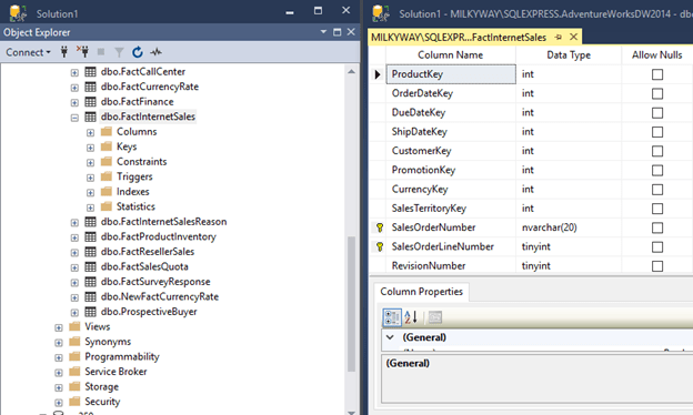
Step-3: Locate the Table dbo.FactInternetSales
This database has a number of tables to populate Power BI with the sample data.
We will be using the FactInternetSale table.
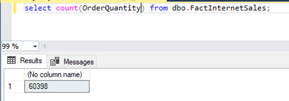
Step-4: Retrieve the total number of the records
Issue select statement to see how many rows in the table.
There are 60,398 records.
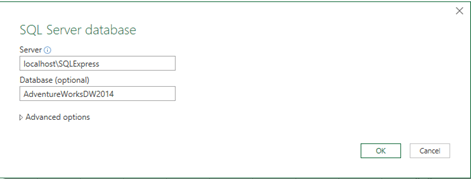
Step-5: Import the Table Content into Excel
Open Up Excel
Click on Data à Get Data à SQL Server.
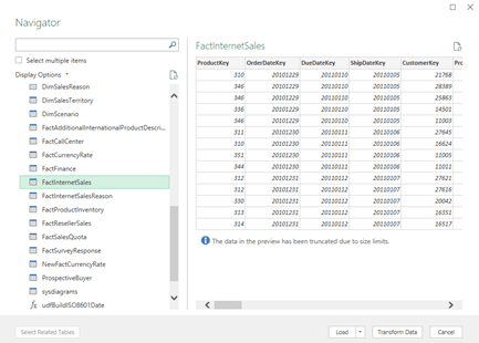
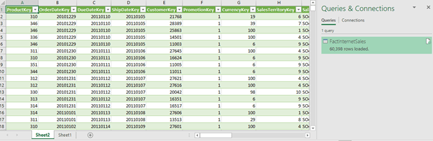
After loading the table in the Excel file, you will get something like the following.
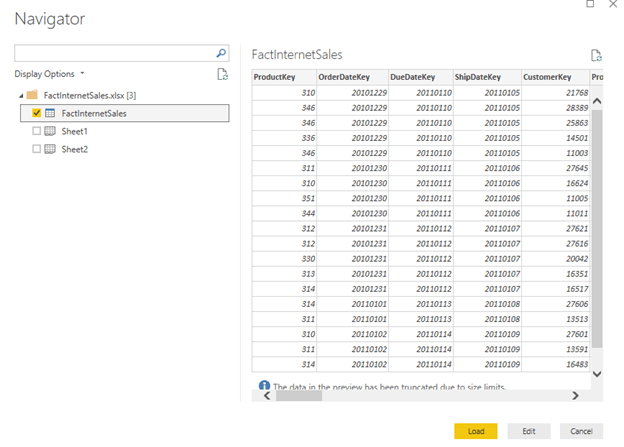
Step-5: Import Excel Into Power BI
Get Data
Select Excel
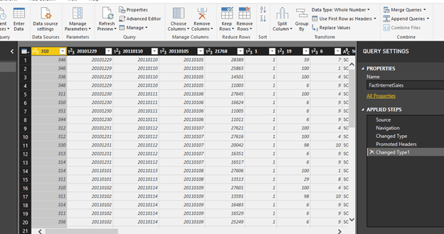
Step-6: Click Edit and Select Use First Row as Header
Click on Load.
Click Close and Apply
Step-7: Select the Desire Fields and Set up Their Properties
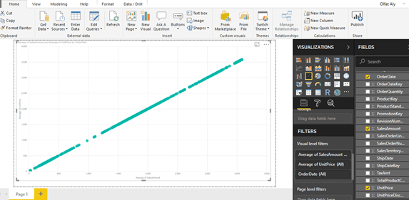
One standard method of analyzing two numerical values on a graph is by using scatterplot graph.
In a scatterplot graph, each value has an X-axis, and Y-axis is plotted on the graph using the values of two scales.
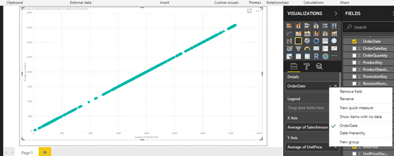
You will use the fields as Average of UnitPrice and Average of SalesAmount.
You also want to see this comparison over time, so you will add the OrderDate field in the Details section.
Select OrderDate, SalesAmount, UnitPrice.
Select Average of SalesAmount.
Select Average of UnitPrice.
Select OrderDate from OrderDate instead of Date Hierarchy.
Select the scatterplot icon from the visualizations pane and create a blank scatterplot graph on the report layout.
Select his blank graph, and add the fields as discussed above.
This will create a scatterplot chart of average of unit price vs. average of sales amount over time.
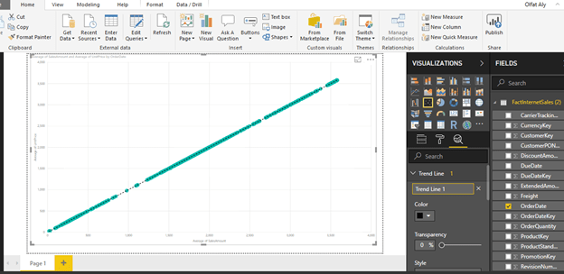
Step-8: Add a Trend Line
The chart seems to show linear relationship as the points seems to be organized in a straight line, but you cannot be sure just by reviewing visually.
The chart seems to show a series of points that are closely overlaid near or on the top of each other.
You need an explicit indicator of the same, like a project trend line in the graph.
To accomplish the same, click on Analytics Icon/Pane and you should find a trend-line option as shown below.
Click and Add to create a new trend line.
You can format the different options as shown below.
After adding the trend line, the graph should look as shown below.
This looks very trivial as you can create a trend using a line chart.
However, this trend is more like a linear trend line used in a linear regression method where the best-fit line passes through the minimum of squares distance/variance from all the points in the plot.
Linear regression analysis is part of statistical analysis which is part of machine learning techniques.
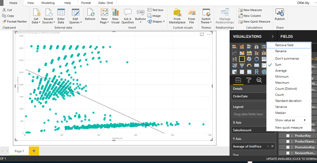
Step-9: Use Different Aggregation instead of Average Sales
You can try a different aggregation to look at a different trend.
Instead of the average of Sales Amount, change the aggregation to Sum of the Sales Amount.
To change the aggregation, you need to right-click on the field, and select the aggregation of choice from the menu as shown below.
Select Sum for Sales Amount
After making the change, the trend would look as shown below.
This shows that the trend is negative.
As the average of unit price decreases, the sum of sales amount increases.
From this limited trend analysis, without looking at the data, you can make an initial assumption that as the average of unit price of products increases, the sum total of overall sales decreases, but the average of sales increases.
This indicates that for expensive products the total sales is low.
As the number of products sold are less and the unit price is high, the average keeps on increasing shown a linear positive trend.
In this way, trend line enables quick interpretation of the data using different aggregations with trend lines.
The purpose of this project is to analyze a dataset using the correlation analysis and correlation plot in PowerBI.
Correlation Analysis is a fundamental method of exploratory data analysis to find a relationship between different attributes in a dataset.
Statistically, correlation can be quantified by means of a correlation coefficient, typically referred as Pearson’s co-efficient which is always in the range of -1 to +1.
A value of -1 indicates a total negative relationship and +1 indicates a total positive relationship.
Any number closer to zero represents very low or no relationship at all. There is a statistical calculation involved to find this co-efficient and using this you can identify the correlation between two attributes with numerical data.
It can be a very statistically intensive process if the task is to identify correlation between many numeric variables.
Correlation plots can be used to quickly calculate the correlation coefficients without dealing with a lot of statistics, effectively helping to identify correlations in a dataset.
Step-by-Step Instruction
Step-1: Install the R Package for Correlation Plot
Power BI provides correlation plot visualization in the Power BI Visuals Gallery to create Correlation Plots for correlation analysis.
In this tip we will create a correlation plot in Power BI Desktop using a sample dataset of car performance. It is assumed that Power BI Desktop is already installed on your development machine. So please follow the steps as mentioned below.
This visualization makes using of the R “corrplot” package. The same plot can be generated using the R Script visualization and some code. Instead this visualization eliminates the need for coding and provides parameters to configure the visualization.
The first step is to download the correlation plot
Install the R correlation package.
From the File à Import à custom visual from marketplace
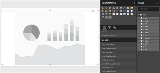
Step-2: Expand the correlation plot to the entire area
After the correlation plot is added to the report layout, enlarge it to occupy the entire available area on the report. After you have done this, the interface should look as shown below.
Step 3: Download the CSV file (cars.csv)
Now that you have the visualization, it is time to populate it with some data on which correlation analysis can be performed.
You need a dataset with many numerical attributes.
The file contains data on car performance with metrics like
miles per gallon,
horsepower,
transmission,
acceleration,
cylinder,
displacement,
weight,
gears, etc.
Click on the Get Data menu and select CSV since we have the data in a csv file format.
Step-4: Edit the file and select “Use First Row as Header”
This will open a dialog box to select the file.
Navigate to the downloaded file and select it.
This will read a few records from the file and show a data preview as shown below.
The column headers are in the first row.
Click on the edit button to indicate this before importing the dataset.
Click on the “Use First Row as Headers” to get the column names properly.
You can also rename the Car Names column and name it Model.
Step-5: Apply the changes
After you apply the setting, the column names should look as shown below.
Click on the Close and Apply button to complete the import process.
Step-6: Import the data into the Power BI Desktop
The model should look as shown below.
Select the fields and add them to the visualization.
Click on the visualization in the report layout and add all the fields from the model except the model field which is a categorical / textual field.
The visualization would look as shown below.
Step-7: Points for consideration when reading the plot
The dark blue circles in a diagonal line from top left to bottom right shows correlation of an attribute with itself, which is always the strongest or 1. So this should not be read as correlation, but just as a separator line.
The more the circle has a dark blue color, it signifies stronger positive correlation. The darker the red color, it signifies a negative correlation. Lighter or white colors signifies weak or no correlation.
The scale can be used to estimate the correlation coefficient value.
Step-8: A Few Modifications in the Plot to Make it Visually Analyzable
Make a few modifications in this plot to make it visually analyzable.
Click on the Format option, in the Labels section and increase the font size, so that the field labels are clearly visible as shown below.
As you can see, weight (wt) has a strong positive correlation with displacement (disp) and miles per gallon (mpg) has a strong negative correlation with weight (wt).
The data is shown in a matrix format and there are many positive and negative correlation spreads in the plot.
Step-9: Draw a Cluster
It would be easier to analyze correlation if attributes with the same type of correlation are clustered together.
To do so, select the correlation plot parameters and set the “Draw clusters” property to “Auto”. This will cluster and reorganize the attributes as shown below.
Step-10: Add Number for Easy Analysis
The strength of the correlation is still shown by the depth of the color.
It would be easier to analyze the data if it is shown by a number indicating this strength – i.e. correlation coefficient.
To do so, switch On the Correlation Coefficients section and increase the font size, so that you can see the coefficient clearly.
Using the values as a reference, you can easily find out the strongest and weakest correlation in the entire dataset.
There are other sections for formatting the data, but those are mostly related to cosmetic aspects of the plot like title, background, transparency, title, etc.
You can try to modify those settings and make the plot more suitable to the theme of the report.
You can add Title from the Format section.
With Power BI, without digging into any coding or complex statistical calculations, one can derive correlation analysis from the data by using the correlation plot in Power BI Desktop.
The purpose of this projectis to discuss the trade-off between cost, time and quality of projects. Various essential topics related to projects and project management are discussed. The discussion begins with the distinct characteristics of the projects and operations, among which projects are temporary while operations are repetitive. The project addressed the project cycle plan and project development tools. Various tools for project management include project evaluation and review techniques (PERT), critical path method (CPM) and Gantt Chart. The project management with the trade-off between time, cost and quality are addressed. A balance of these three critical elements is required. This project discusses the project trade-off and the correlation between time and cost. Some argue that most businesses are cost-time bias at the expense of quality. Various projects success factors are also discussed in this project. Various factors cause projects to fail. These factors include misunderstanding of the project requirement, organizational influences, and risk management. Failed projects take a long time to be abandoned or corrected due to logistical problems, political thinking and lack of planning for uncertainty, and risk management.
Keywords:
Project Management, Cost, Time, Quality.
Enterprises achieve their strategic goals using various project
management techniques. Business requires
good performance assessment tools for project management to make sound decision
to gain and maintain a competitive edge in the market (Anuar & Ng, 2011). Management
and executives are under pressure to complete projects within a specific time, a
specific budget while maintaining the quality, which is considered to be the
success factors for project implementation.
This project discusses these factors for project management. It begins
with the discussion of projects vs. operations, followed by the project cycle
plan and project development tools.
A project is defined as a temporary venture to implement
a unique service or product. The temporary indicates a period that has a
beginning and ending, while unique indicates the service or product will be
distinguished from the ones in the market (Pearlson & Saunders, 2001; PMI, 2000). It is also defined as an
organization of people dedicated to a specific purpose or object (Pinto & Slevin, 2015). Projects consist of a set of
one-time actions to shift the present event into a new one based on the
strategic plan of the enterprise (Pearlson & Saunders, 2001; PMI, 2000). Projects involve substantial, expensive,
unique or high risk and must be completed within a time frame using a certain
amount of investment (Pinto & Slevin, 2015). Projects need to have
well-identified objectives and sufficient resources to implement all the
required tasks and activities (Pearlson & Saunders, 2001; PMI, 2000). The successful strategy of the enterprise requires two types of decisions;
one for the daily operatives, and another for the strategic objectives. Since IT plays a significant role in all
projects of the enterprise, IT project management plays a critical role in the
success of the business.
Projects and operations utilize the resources of the
business to transform them into profits.
Human resources and the flow of resources are required for projects and
operations of the business. A project
can be divided into sub-projects to implement particular activities such as
quality control testing (Pearlson & Saunders, 2001). During this sub-division of a
project, sourcing decisions are made to limit costs. Various projects are organized at a high
level, and elements of a more extensive program which provide a framework from
which competing resource requirements are managed, and priorities among a set
of projects are shifted.
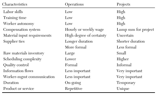
Projects and operations have the same elements such as labor skills, training time, worker autonomy, compensation system, material input requirements, supplier ties, raw materials inventory, scheduling complexity, quality control, information flows, worker-management communication, duration and product or service (Pearlson & Saunders, 2001). However, each element has a different characteristic of the project and the operation. For instance, operations require low labor skills, training time, worker autonomy, while projects require them high. Compensation is a lump sum for projects, while hourly or weekly wage for operations. Material input requirements for operations require a high degree of certainty, while projects are uncertain. Information flows, and worker-management communication is essential in projects, while less critical in operations. The duration is on-going for operations, while temporary for projects. The product or service is repetitive in operation, while unique in projects. Table 1 shows the characteristics of operations and projects (Pearlson & Saunders, 2001).
Table 1. Projects vs. Operations (Pearlson & Saunders, 2001).
Enterprises develop the operations of the business
based on a strategic plan that has goals and objectives (Wilson, 2015). Resources get
acquired and managed to implement the plan. The project plan is comprised of
sequential steps for organizing and tracking the work of the team which
implements the project, while the project management contains a set of tools to
balance the competing demands for resources and ensure the completion of the
work at every step and evolves throughout the project plan (Pearlson & Saunders, 2001).
The project cycle plan organizes
the activities of the project and sequences them in steps along a timeline so
that the project delivers based on the requirements of the stakeholders and
customers. The plan is bounded by a critical beginning and end dates and breaks
the work into phases (Pearlson & Saunders, 2001). The plan
identifies the resources and time required to complete the work based on the
scope of the project. The tasks are identified and assigned to team members. The management tracks the progress and the
phases of the project and coordinates the eventual transition from the project
to operational status, a project that leads to the milestone of the project by
delivering it. The project progress is
monitored to ensure it meets the requirements of the cost, time, and
quality. If the project does not meet
the requirements, some corrections must be made, and the cycle gets adjusted as
required (Copertari, 2002; Pearlson & Saunders, 2001).
Various approaches and
software tools exist for the development of the project. Three main approaches include project evaluation
and review techniques (PERT), critical path method (CPM), and Gantt Chart (Pearlson & Saunders, 2001). PERT method
identifies the tasks of the project, orders the tasks in a time sequence,
identifies the interdependencies of the tasks, and estimates the time which is required
to complete each task. Tasks are divided
into critical and non-critical. The critical tasks must be performed
individually and together impact the total elapsed time of the project, while
the non-critical tasks include slack time without impacting the duration of the
entire project. Figure 1 shows an example of a PERT chart for a project plan.
Figure 1. PERT Chart (Pearlson & Saunders, 2001).
The CPM is another project planning and scheduling
tools. CPM is similar to PERT. However,
unlike PERT, CPM can identify relationships between costs and completion date
of a project, the amount and value of resources which can be applied as
alternatives (Pearlson & Saunders, 2001). CPM and PERT
are different in term of time estimates.
PERT develops broad estimates about the time needed to complete the
tasks of the project, calculating the optimistic, most probable and pessimistic
time estimates for each task. CPC, in
contrast, assumes that all time requirements for completion of each task are
relatively predictable. CPM tends to be
used on projects for which direct relationships can be established between time
and costs.
Gantt charts are used mostly for displaying time relationships of the tasks of the project and for monitoring the progress toward project completion. Gantt charts list project task with a bar for each task indicating the relative amount of time expected to complete the task (Pearlson & Saunders, 2001). The due date for completion is regarded as a milestone and noted with diamonds. Gantt charts are useful for planning purpose at the beginning of the project. When the project progresses, the chart is altered to reflect the extent to which each task is completed at the time the project is monitored. Figure 2 illustrates an example of a Gantt chart for a project.
Project management is defined as the application of skills, knowledge, techniques, and tools to implement activities to meet or exceed the needs of the stakeholders and the expectation from a project (Pearlson & Saunders, 2001). Project management involves a continuous trade-off between cost, quality and time. Managers and executives are confronted with a serious decision among these triangle constraints for projects implementation, involving the scope of the project. The scope can be divided into product scope and project scope. The product scope includes a detailed description of the quality of the product, features, and functions, while the project scope involves the work required to deliver a product or service with the intended product scope. Time refers to the period that is required to complete a project, while cost involves all the required resources to implement the project. Figure 3 shows the triangle of project management.
Any modification in any of these three sides of the
project triangle can have an impact on either side or both of the other sides. For instance, if the scope of the project
increases, more time and more cost will be required to implement the additional
work. The increase in the scope after
the project started is known as scope
creep. One or two of these project
triangle elements can be optimized, modifying the third to maintain the
balance. For instance, a project with a
fixed time and a fixed budget can restrict the scope, while a project with a
short time and a broad scope need budget flexibility. The trade-off among these project elements plays
a crucial role in business, as it can lead to a disastrous event such as Titanic.
The use of substandard low-grade rivets makes ships sink when hitting an
iceberg. The history showed that the
quality trade-off to using these low-grade reverts to lower the cost of some
parts of Titanic causes a disastrous
event. Managers and executives are under
pressure to balance among these project elements to ensure the success of the
project and eventually the success of the business.
The nature of the underlying tradeoffs can be illustrated using a systematic approach (Copertari, 2002). The systematic relationship between time and cost is illustrated in Figure 4 (a). If the project is delayed, it costs more money which is supported by studies such as (Anuar & Ng, 2011; Atkinson, 1999; Bowen, Cattel, Hall, Edwards, & Pearl, 2012). This relationship is a positive correlation between time and cost. Additional resources are required to deliver on time which can be directed to critical activities. Limited resources should be directed to non-critical activities, which is called crashing and it has a negative correlation between cost and time. The nature of the activities as critical and non-critical and the existing of both positive and negative correlation implies the existence of an equilibrium where an optimal project completion time is achieved at a minimum cost. Figure 4 (b) illustrates how the time/cost tradeoff is influenced by performance. The quality can be improved by using more resources, which increases the financial cost and will increase the time if such resources are limited. However, if more resources are invested and the project is taken more time to complete, the cost increases, the Internal Rate of Return (IRR) of the project measuring the profitability is reduced. Thus, enterprises must maintain an optimal time/cost tradeoff that can yield optimal project performance as measured by its IRR (Copertari, 2002).
Figure 4. Time, Cost and Performance
Tradeoffs (Copertari, 2002).
Various studies discussed various factors affecting
the success of projects. (Thamhain, 2004) examined the influences of the project environment on
team performance. The result showed that
a general agreement existed on the factors that drive team performance, and a
large number of performance factors derived from the human side is the most
significant findings. Project success is
based on the effectiveness of multi-disciplinary efforts across various teams (Thamhain, 2004). (Hong, 2011) suggested that the initiation and planning phases of
capital projects impact the outcome of completed cost, time and
profitability. (Bonner, Ruekert, & Walker Jr, 2002) examined formal and interactive control mechanisms
available to upper-managers in controlling new product development (NDP)
projects, and the relationship between these techniques and the NDP project
performance. The findings indicated that the degree to which upper-management
intervened in project-level during the project was negatively related to
project performance. The results also
showed support for the notion that early and interactive decision-making on
control mechanisms is critical for effective projects.
Other studies discussed cost, time and quality as
success factors for project implementation and management. (Atkinson, 1999) indicated that the Iron Triangle of time, cost, and
quality is still preferred success criteria for projects. Time is an intangible resource binding the
period of the project from the start to the completion (Anuar & Ng, 2011; Pearlson & Saunders, 2001). Time plays a significant role in the success
of the project as it is regarded as a significant criterion for project success
(Anuar & Ng, 2011; Bowen et al., 2012). The longer
the project takes, the potential damage is expected, the more complex and
costly the corrective measures will be to the project. Some argue that the projects with a short
time frame for completion have advantages cost and performance wise, while
others argue that when the projects are under time and cost pressure, the
quality is profoundly affected (Anuar & Ng, 2011; Pollack-Johnson &
Liberatore, 2006). (Bowen et al., 2012) suggested that time-cost bias exist, indicating
quality is last to consider.
Every project requires financial resources reflecting
the costs. The cost of the project plays another significant role in the
success of projects implementation (Westland, 2018; Wilson, 2015). Some suggest that when the cost increases when the
duration is shortened, and vice versa.
However, most large and complex project development require substantial
financial resources and schedule overrun (Anuar & Ng, 2011). The delayed
and more time projects require more financial resources (Bowen et al., 2012; Shankar, Raju, Srikanth, &
Bindu, 2014).
Products or service without quality can bring a business
down. Quality is defined as one of the
components that contribute to value for money (Bowen et al., 2012). Enterprises
must pay attention to the quality of products and services. The high failure rates of quality suggest
that the knowledge of the transformation process whereby ideas are turned into
successful quality products and services is far from perfect (Anuar & Ng, 2011). Organizations
are under pressure to introduce new products and adopt new processes to gain
and maintain competitive advantages.
(Anuar & Ng, 2011) analyzed three different scenarios and modeling using
Microsoft Office Project tool. The first
scenario is about project fixed time with limited resources. The second scenario is about project time
reduced with minimus cost imposed. The
last scenario is about maintaining quality while reducing the project
duration. The findings of the first
scenario showed that cost was controlled very tightly even though the time of
the project was not required to be reduced.
These findings are similar to the findings of (Olson, Walker Jr, Ruekerf, & Bonnerd, 2001). The findings
of the second scenario showed that the reduced time of the project could reduce
the cost of the project. The findings of
the last scenario showed that a shorter duration was not considered due to the
risks of having quality issues (Nidumolu, 1996) argued that the tight control of the process could
result in strict adherence to time and cost estimates. Such control impacts the functionality of the
product, thereby the long-term flexibility of technology is jeopardized with
the short-term user needs.
Various studies discussed reasons for projects
management failure. (Atkinson, 1999) identified two types of errors for project failure;
Type I and Type II. Type I errors occur
when something is done wrong, while Type II errors occur when something has not
been done as well as it could have been or something was missed. (Gardiner & Stewart, 2000) examined the relationship between project budgets,
cash flow cost control and schedule.
Each element plays a significant role in the net present value (NPV) of
a project. The NPV can be used as a
technique to monitor the health of the project, and whether it is meeting the
objectives within the time and cost identified.
The failure of a project is measured by the net present value (Gardiner & Stewart, 2000).
When a project absorbs a delay to a deliverable on the
critical path, five options are available (Gardiner & Stewart, 2000). The first
option is to move the milestone date. The second option is to reduce the scope
of the deliverable. The third option is to reduce the quality of the
deliverable. The fourth option is to apply additional resources generally workforce
or money. The last option is to
rearrange the workload. However, another
investment appraisal is not carried in most cases to assist in determining what
the most appropriate action is. The
point is that the logistical problems and political thinking play a role within
a project and the project managers should not ignore these facts. These logistical problems and political
thinkings play a role in taking a long time in abandoning a project or
correcting a project (Gardiner & Stewart, 2000).
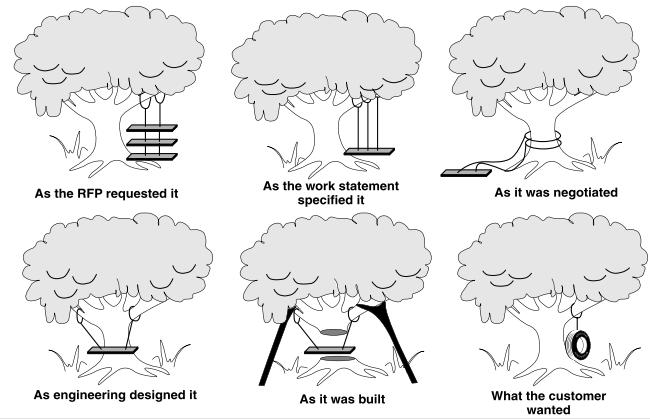
Understanding the requirement of the project play a significant role in the success of the project. Thus, the lack of understanding of the requirements of the project can lead to a different outcome, delayed project, or failed project (Forsberg, Mooz, & Cotterman, 2000). The requirement of a project begins with the customer’s needs, and not with the perception of the organization to the customer’s needs. There is an ongoing danger of misunderstanding and ambiguity in the end-to-end chain of technical, business and project development. This misunderstanding leads to non-essential, overspecified, unclear or missing requirements as illustrated in Figure 5, which is a cartoon. Such projects are subject to failure.
Figure 5. Misunderstanding Project
Requirements Leads to Project Failure (Forsberg et al., 2000).
Moreover, project managers are confronted with various
influencing factors including technical, organizational, and socioeconomic
influences, which are relatively unique to IT projects (Pearlson & Saunders, 2001). Technical issues are related to business and budget
issues. Management which does not feel
comfortable with technology often take one of these actions; either ignore the
IT issues or delegate them to information system organization or focus
inappropriate attention on managing the technology to counter their fear. The managerial and socioeconomic influence involves
the control systems used for non-project-based operations which do not efficiently
support the project management. The
organizational culture has an impact on the leadership style of the project
management, and communication between team members. The socioeconomic impact on
projects includes government and industry standards, globalization, and
cultural issue.
The IT projects have a higher risk than non-IT
projects (Pearlson & Saunders, 2001). The term risk is not well understood among various
project management. The risk is defined as the possibility of the additional
cost or loss due to the alternatives are chosen. Some alternative has a lower risk than
others. Risk can be measured and
quantified by assigning a probability of occurrence and a financial consequence
to each alternative. Risk involves
complexity, clarity, and size (Pearlson & Saunders, 2001). The more
complexity of the project, the higher is the risk associated with the
project. The more ambiguous the project,
the higher the risk, and the bigger the size or scope of the project, the higher
is the risk. There is a positive
correlation between risk and these three risk elements.
The management of these risks can aid in turning the
troubled projects into a successful one.
(Pearlson & Saunders, 2001) argued that trouble projects persist long before they
get abandoned. The amount of money invested on the trouble project biases
management toward continuing to fund the project even if the success of the
project is questionable. Other factors
include the penalties for failure within the organization that can be high;
project management is willing to go for a more extended period even if it means
more resources including cost. Emotional
attachment to the project can cause prolonged projects that are subject to
failure.
This project
discussed various essential topics
related to projects and project management.
It began with the unique
characteristics of the projects and operations, among which projects are
temporary while operations are repetitive.
The project cycle plan and project development tools are also discussed.
Various tools for project management were also discussed. These
tools include project evaluation and review techniques (PERT), critical path
method (CPM) and Gantt Chart. Project
management involves various elements including cost, time and quality. The
project also discussed project trade-off
and the correlation between time and cost.
Some argue that most businesses are cost-time bias at the expense of
quality. Various projects success
factors were also discussed in this project,
such as the balance between cost, time and quality. Various factors cause projects to fail. These
factors include misunderstanding of the project requirement, organizational
influences, and risk management. Failed projects take a long time to be abandoned or corrected due to logistical problems,
political thinking and lack of planning for uncertainty. Although the success of a project is
questionable, the management persists in implementing, and it takes a long time
before it gets abandoned or to put under control. Various factors contribute to
this phenomenon including the penalty for failing projects, lack of
understanding to risk management, and the emotional attachment to the
project.
Anuar, N. I., & Ng, P. K. (2011). The role of time, cost and quality in
project management. Paper presented at the Industrial Engineering and
Engineering Management (IEEM), 2011 IEEE International Conference on.
Atkinson,
R. (1999). Project management: cost, time and quality, two best guesses and a
phenomenon, its time to accept other success criteria. International journal of project management, 17(6), 337-342.
Bonner,
J. M., Ruekert, R. W., & Walker Jr, O. C. (2002). Upper management control
of new product development projects and project performance. Journal of Product Innovation Management: AN
INTERNATIONAL PUBLICATION OF THE PRODUCT DEVELOPMENT & MANAGEMENT
ASSOCIATION, 19(3), 233-245.
Bowen,
P., Cattel, K., Hall, K., Edwards, P., & Pearl, R. (2012). Perceptions of
time, cost and quality management on building projects. Construction Economics and Building, 2(2), 48-56.
Copertari,
L. F. (2002). Time, cost and performance
tradeoffs in project management.
Forsberg,
K., Mooz, H., & Cotterman, H. (2000). Visualizing
project management: a model for business and professional sucess: John
Wiley and Sons.
Gardiner,
P. D., & Stewart, K. (2000). Revisiting the golden triangle of cost, time
and quality: the role of NPV in project control, success and failure. International journal of project management,
18(4), 251-256.
Hong,
L. C. (2011). Predictors of project performance and the likelihood of project
success.
Nidumolu,
S. R. (1996). Standardization, requirements uncertainty and software project
performance. Information &
Management, 31(3), 135-150.
Olson,
E. M., Walker Jr, O. C., Ruekerf, R. W., & Bonnerd, J. M. (2001). Patterns
of cooperation during new product development among marketing, operations, and
R&D: Implications for project performance. Journal of Product Innovation Management: An International Publication
of the Product Development & Management Association, 18(4), 258-271.
Pearlson,
K., & Saunders, C. (2001). Managing and Using Information Systems: A
Strategic Approach. 2001: USA: John Wiley & Sons.
Pinto,
J. K., & Slevin, D. P. (2015). 20. Critical Success Factors in Effective
Project implementation*.
PMI.
(2000). Project management body of
knowledge (PMBOK).
Pollack-Johnson,
B., & Liberatore, M. J. (2006). Incorporating quality considerations into
project time/cost tradeoff analysis and decision making. IEEE Transactions on engineering management, 53(4), 534-542.
Shankar,
N. R., Raju, M., Srikanth, G., & Bindu, P. H. (2014). Time, cost and
quality trade-off analysis in the construction of projects.
Thamhain,
H. J. (2004). Linkages of the project environment to performance: lessons for
team leadership. International journal of
project management, 22(7), 533-544.
Westland,
J. (2018). The Triple Constraint in Project Management: Time, Scope & Cost.
Wilson, R. (2015). Mastering
Project Time Management, Cost Control, and Quality Management: Proven Methods
for Controlling the Three Elements that Define Project Deliverables: FT
Press.